How to build an Anomaly Detector using BigQuery
Chloé Caron15 min read

Bad data quality can arise in any type of data, be it numerical, textual or other. As we saw in the last article of this series, LLMs like OpenAI are quite effective at detecting anomalies in textual data. However, the OpenAI anomaly detector really struggled with numerical data, reaching an accuracy of 68% even after applying multiple forms of prompt engineering (compared to ~100% for textual data).
This is to be expected since OpenAI is a large language model and isn’t trained on mathematical concepts. What to do? Numerical data is a non-negligible proportion of global data. Although not backed by exact statistics, it wouldn’t be an unreasonable statement to say that the proportion of data which is numeric is bigger than that which is textual. A few sources could include scientific, financial, market and consumer, sensor, healthcare data, etc., the list is endless.
So if we can’t use LLMs to build our anomaly detector, what do we use? BigQuery ML is one solution to our problem! BigQuery ML has an inbuilt ‘anomaly detector’ function which we can use to identify anomalies in our data. Let’s give it a shot and work through this together.
Part 1: Choosing and preparing a model
Before we try to detect any anomaly in our data, we need to create a model that our anomaly detector will base itself off of, i.e. does your dataset match what the model predicted?
Choosing the correct model is important based on your situation. To help understand the differences between the type of models and choose the correct one, I built this decision tree:
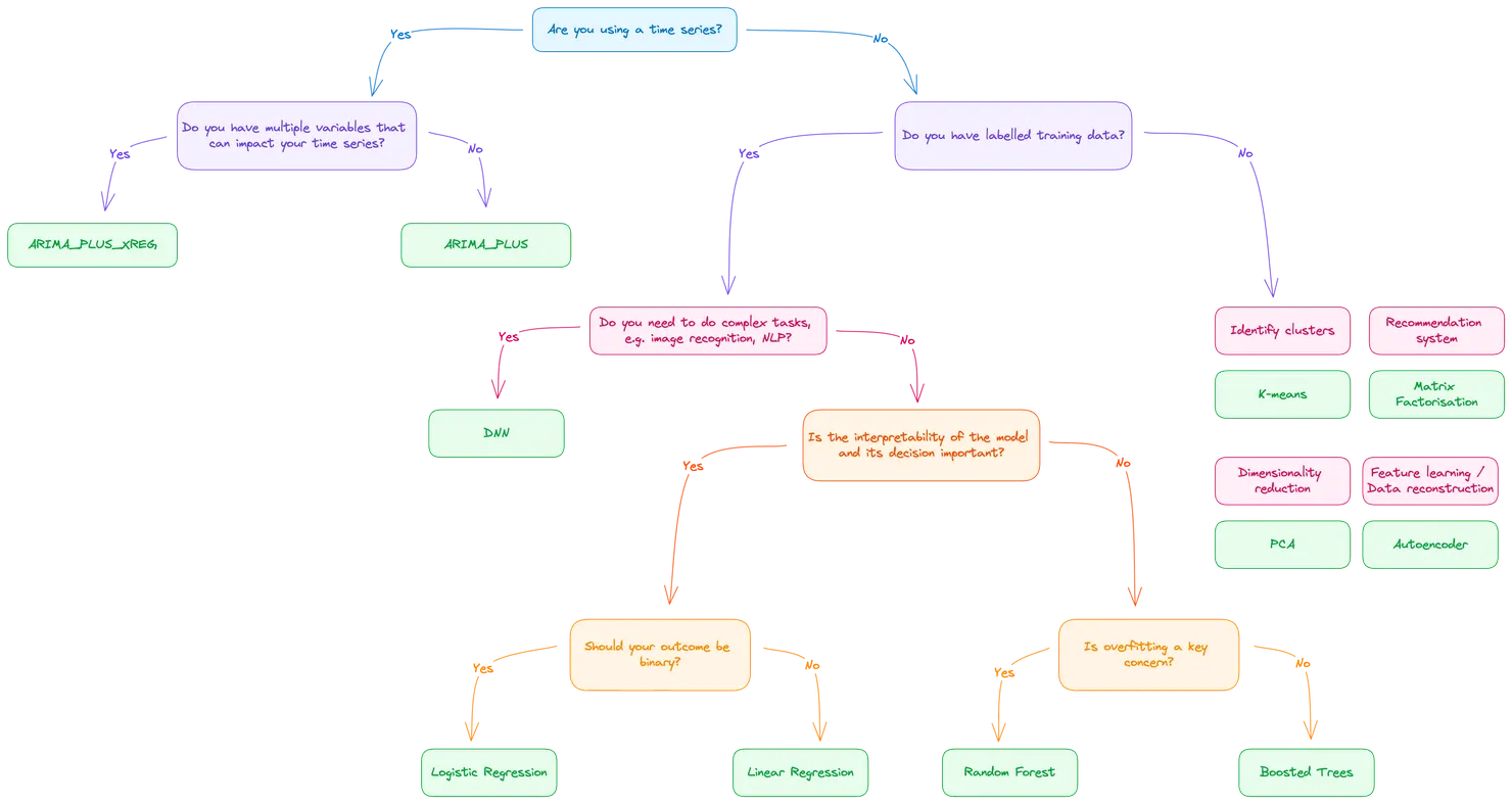
If you remember from my previous article, we are using data from the Electricity Consumption UK 2009-2023 dataset.
The data we have is a time series and, for our case scenario, we’ll keep it simple and not look at cross dependencies between variables (although this would be an interesting experiment to try). Our logical choice is, therefore, to use ARIMA_PLUS as our model type. If you would like to know more about the ARIMA_PLUS model, don’t hesitate to have a look at BigQuery’s documentation!
Going back to our dataset, you can notice that we have a lot of data columns, i.e. for a singular timestamp we are collecting multiple types of data (e.g. wind generation, solar generation). These can’t all fit into a single model. An ARIMA_PLUS model can only point to a single data column and be trained on that column. In this case, we’ll need to create a separate model for each data column that we have.
If you haven’t worked with BigQuery before, have a look at some of the tutorials online. This one is a relatively good start and you just need to know how to upload data using a CSV (or other) and how to run a query before being able to follow through these steps.
Okay, great! So we know that we’ll be using the ARIMA_PLUS model, we know what data we want to use and we know that we’ll need a model per column. Let’s see this in action as a query.
DECLARE column_names ARRAY<STRING>;

DECLARE column_name STRING;
DECLARE query_string STRING;

-- Get column names into an array
SET column_names = (
  SELECT ARRAY_AGG(COLUMN_NAME)
  FROM `project-name.dataset-name.INFORMATION_SCHEMA.COLUMNS`
  WHERE TABLE_NAME = 'name_of_your_table_with_data' AND COLUMN_NAME != 'name_of_your_column_with_your_timestamp'
);

-- Loop through columns and create ARIMA_PLUS models
FOR row IN (SELECT * FROM UNNEST(column_names) AS column_name)
DO
    SET column_name = row.column_name;

    SET query_string = (
    SELECT
      'CREATE OR REPLACE MODEL `dataset-name.data_arima_model_' || column_name || '` ' ||
      'OPTIONS(MODEL_TYPE="ARIMA_PLUS", TIME_SERIES_DATA_COL="' || column_name || '", TIME_SERIES_TIMESTAMP_COL="name_of_your_column_with_your_timestamp") AS ' ||
      'SELECT name_of_your_column_with_your_timestamp, ' || column_name || ' FROM `project-name.dataset-name.table-with-data`'
  );

  EXECUTE IMMEDIATE query_string;
END FOR;
Let’s break this down. In the first section, we are creating an array of the column names (remember to replace project-name, dataset-name, name_of_your_table_with_data, table-with-data and name_of_your_column_with_your_timestamp with your own values). This array is used in the next section where we loop through them and create an individual ARIMA_PLUS model for each data column.
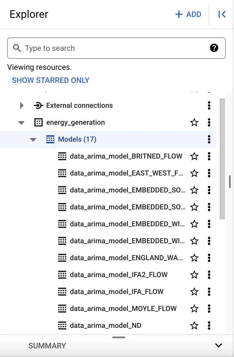
Great, we have our models! Once the query has run and if it’s successful, you’ll be able to see the models in the explorer tab within the GCP console:
(Optional) Formatting your timestamp
If you use the same dataset that I did (Electricity Consumption UK 2009-2023 dataset), you’ll notice that you don’t quite get a good timestamp. Instead you have SETTLEMENT_DATA and SETTLEMENT_PERIOD to determine which half-hour period of the day you are in. As is, this will cause an error when you run your model since the TIME_SERIES_TIMESTAMP_COL that you will try to use will not be a timestamp.
But, no worries, I have a script to solve that!
Once you’ve imported your data, run the following script:
-- Step 1: Create a new table with the desired structure and transformed data
CREATE OR REPLACE TABLE `project-name.dataset-name.<table-with-data>_new` AS
SELECT
  * EXCEPT (SETTLEMENT_DATE, SETTLEMENT_PERIOD),  -- Exclude the columns you want to remove
  DATETIME(CONCAT(FORMAT_DATE('%F', SETTLEMENT_DATE), 'T',
    CASE
      WHEN SETTLEMENT_PERIOD = 48 THEN '00:00:00'
      WHEN SETTLEMENT_PERIOD < 20 THEN CONCAT('0', CAST(FLOOR((SETTLEMENT_PERIOD) / 2) AS STRING), ':', LPAD(CAST(MOD(SETTLEMENT_PERIOD, 2) * 30 AS STRING), 2, '0'), ':00')
      ELSE CONCAT(CAST(FLOOR((SETTLEMENT_PERIOD) / 2) AS STRING), ':', LPAD(CAST(MOD(SETTLEMENT_PERIOD, 2) * 30 AS STRING), 2, '0'), ':00')
    END)) AS time_stamp
FROM `project-name.dataset-name.table-with-data`;

-- Step 2: Drop the original table
DROP TABLE `project-name.dataset-name.table-with-data`;

-- Step 3: Rename the new table to the original table name
ALTER TABLE `project-name.dataset-name.<table-with-data>_new` RENAME TO `table-with-data`;
This is where the magic of SQL comes in so I would highly recommend looking over this script to make sure you understand each stage.
Part 2: Setting up our results table
Now that our models have been generated, we are nearly ready to run our anomaly detector. But, what’s the point in running the experiment if we can’t see the data? And what is the easiest and most pragmatic way to visualise that data? We’re in the data world, so we can talk about all sorts of beautiful visualisations, but let’s keep it simple with storing our results in a table. First, let’s prepare the table:
DECLARE dynamic_sql STRING;
DECLARE column_name STRING;

-- ... the code to set the column_names, seen above, is needed again

-- Start building the dynamic SQL to create the table of results
SET dynamic_sql = 'CREATE OR REPLACE TABLE `project-name.dataset-name.anomaly_results` (time_stamp TIMESTAMP, ';

-- Loop through the column names
FOR row IN (SELECT * FROM UNNEST(column_names) AS column_name)
DO
    SET column_name = row.column_name;
    SET dynamic_sql = dynamic_sql || column_name || ' FLOAT64 DEFAULT NULL, is_anomaly_' || column_name || ' BOOL DEFAULT FALSE, prob_' || column_name || ' FLOAT64 DEFAULT NULL, ';
END FOR;

-- Remove the trailing comma and close the SQL statement
SET dynamic_sql = SUBSTR(dynamic_sql, 1, LENGTH(dynamic_sql) - 2) || ')';

-- Execute the dynamic SQL to create the table to store results
EXECUTE IMMEDIATE dynamic_sql;
In this snippet of code, we are creating an empty table and creating 3 columns for each of the original data column: the original data (float64), whether or not the value is an anomaly is_anomaly_<column-name> (bool), and the probability of it being an anomaly prob_<column-name> (float64) which will come in useful for debugging. The default values are quite important to have here. When we are writing to our result table, we will be incrementally adding values to the column as we run our anomaly detector against our models. Since we’ll be adding data to a row in a piece-wise manner, we’ll need to have those default values as placeholders to not get an error when we create a new row with partial data.
Part 3: Running the anomaly detector
Now that we have the model and we have a place to store our results, we can run our anomaly detector.
DECLARE anomaly_column_name STRING;
DECLARE anomaly_prob_column_name STRING;
DECLARE model_name STRING;

-- ... the code to set the column_names, seen above, is needed again

-- Find anomalies in the data
FOR row IN (SELECT * FROM UNNEST(column_names) AS column_name)
DO
  SET column_name = row.column_name;
  SET anomaly_column_name = 'is_anomaly_' || column_name;
  SET model_name = 'dataset-name.data_arima_model_' || column_name;
  SET anomaly_prob_column_name = 'prob_' || column_name;

  SET query_string = (
    SELECT
      'MERGE `project-name.dataset-name.anomaly_results` AS target ' ||
      'USING (' ||
      '  SELECT TIMESTAMP AS time_stamp, ' || column_name || ', is_anomaly AS ' || anomaly_column_name || ', anomaly_probability AS ' || anomaly_prob_column_name ||
      '  FROM ML.DETECT_ANOMALIES(' ||
      '    MODEL `' || model_name || '`, STRUCT(0.95 AS anomaly_prob_threshold)' ||
      '  )' ||
      ') AS source ' ||
      'ON target.time_stamp = source.time_stamp ' ||
      'WHEN MATCHED THEN ' ||
      '  UPDATE SET ' ||
      '    ' || column_name || ' = source.' || column_name || ', ' ||
      '    ' || anomaly_column_name || ' = source.' || anomaly_column_name || ', ' ||
      '    ' || anomaly_prob_column_name || ' = source.' || anomaly_prob_column_name || ' ' ||
      'WHEN NOT MATCHED THEN ' ||
      '  INSERT ' ||
      '    (' || column_name || ', ' || anomaly_column_name || ', ' || anomaly_prob_column_name || ', time_stamp) ' ||
      '  VALUES ' ||
      '    (source.' || column_name || ', source.' || anomaly_column_name || ', source.' || anomaly_prob_column_name || ', source.time_stamp)'
  );
  -- Execute the query
  EXECUTE IMMEDIATE query_string;
END FOR;
This looks like a very complicated statement so let’s break it down again. The first part of the statement is MERGE which will either create, update or delete a row depending on the matching WHEN statement. Here we are determining whether there is a match between the time_stamp in our results table and the one in the data we are going through. The time_stamp was the best choice to see if we needed to update or insert a row since it is unique in our case.
Now that we’ve looked at the MERGE and WHEN statement, let’s look at the USING component which is where we are actually running our anomaly detector. I won’t focus on the query syntax as this ressembles SQL quite closely. The main part of the statement is ML.DETECT_ANOMALIES where we specify the model (which we created earlier) and the probability threshold. This probability threshold is used to determine what the model will mark as an anomaly. The reason behind this is that when this script is run, each piece of data will have a probability of it being an anomaly. If we have a low threshold, we are being more conservative and risk-averse by classifying data as an anomaly if the system is partially sure that the data is anomaly. On the other hand, we could put a much higher threshold and only classify data as an anomaly if the system is near certain (i.e. associates a high probability of being an anomaly).
And that’s it! You’ve manage to run your anomaly detector. 🥳
How good is BigQuery as an anomaly detector?
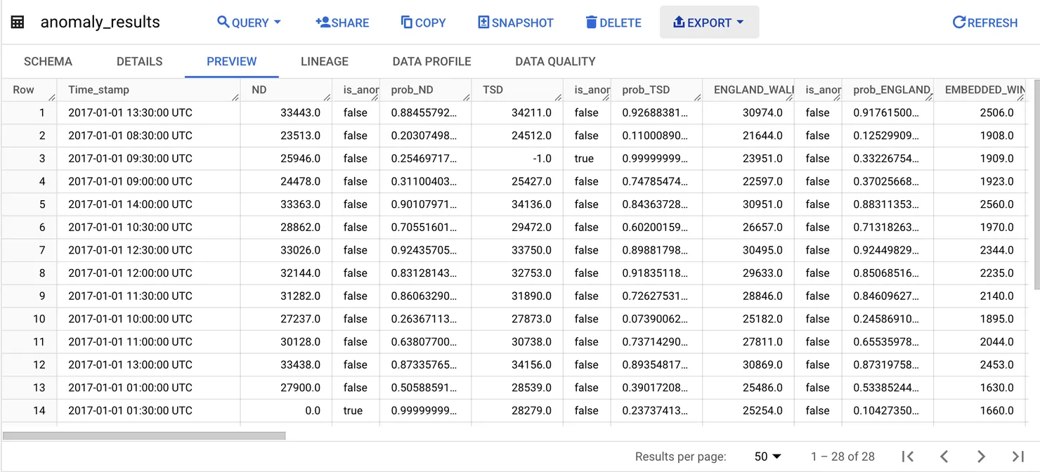
After running the scripts above, you should see that the anomaly_results table has been created with our results. It will look a little like this:
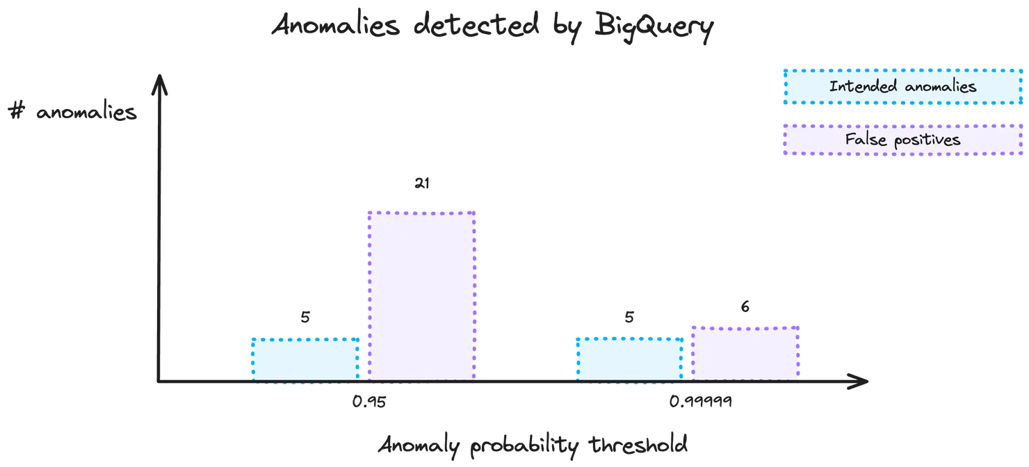
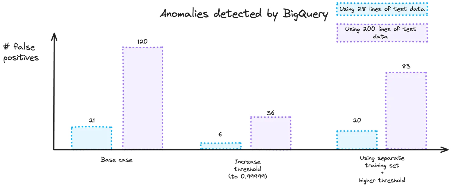
For this test, I used 28 lines of data and introduced 5 anomalies into the data that I imported. What you’ll notice is that BigQuery is very good at picking up the intended anomalies. However, we have a different problem this time. Instead of having issus with picking up the anomalies (which we saw when using an LLM as an anomaly detector in this article), BigQuery has a much bigger issue with false positives. In this first experiment, there were 21 false positives! False positives create a different issue. Although less severe than missing an actual anomaly (which would lead to bad data), false positives can lead to incorrect alerts and the need for a manual verification process, which would hinder an automatic system. So what can we do?
1) Increasing the anomaly probability threshold
When setting up the anomaly detector, there was a short introduction to the probability threshold, i.e. the point at which we consider our data point an anomaly. By raising this threshold, we are essentially saying that we want the system to be more sure a data point is an anomaly before marking it as such. However there is a warning associated to this. The higher you raise the threshold, the higher the risk that you miss an anomaly when the system is less certain about it.
In practise, when raising the threshold from 0.95 to 0.99999, I was pleasantly surprised by the fact that BigQuery still picked up 100% of the intended anomalies. The number of false positives dropped to 6 (-71%) which is a big step in the right direction!
2) Using a separate and more extensive training set
The bigger the training set, the better it performs, right? Not quite in this case. Going with this initial thought process, I trialled using a separate and more extensive training data set to produce the model.
Looking at our code above, it is relatively straightforward to change the dataset which the model is based off of, you just have to update project-name.dataset-name.table-with-data to point to the table with the new data you would like to train the model on.
Next, you’ll also have to update the anomaly detector. If you noticed, in the code above, we don’t specify the data where the anomaly detection is occurring:
'SELECT TIMESTAMP AS time_stamp, ' || column_name || ', is_anomaly AS ' || anomaly_column_name || ', anomaly_probability AS ' || anomaly_prob_column_name ||
'  FROM ML.DETECT_ANOMALIES(' ||
'    MODEL `' || model_name || '`, STRUCT(0.95 AS anomaly_prob_threshold)' ||
'  )' ||
This is because, implicitly, BigQuery uses the same dataset as was used in the model to detect the anomalies. To detect anomalies on a new dataset, you’ll have to modify the line above to have:
'SELECT TIMESTAMP AS time_stamp, ' || column_name || ', is_anomaly AS ' || anomaly_column_name || ', anomaly_probability AS ' || anomaly_prob_column_name ||
'  FROM ML.DETECT_ANOMALIES(' ||
'    MODEL `' || model_name || '`, STRUCT(0.95 AS anomaly_prob_threshold), (SELECT * FROM `dataset-name.table-with-data-to-analyse`)' ||
'  )' ||
where table-with-data-to-analyse is the name of the table which has the anomalies you would like to detect.
Word of warning: the timestamp of your data is important when doing this! The data which you want to analyse has to have a timestamp which is in the future compared to your training data. This makes sense as you use past data to predict future trends and is a design choice that was made by the BigQuery ML team. If you are curious about the reasoning behind this, here is a discussion from within the Google Cloud Community space with more details.
Doing this did not significantly improve the number of false positives. In fact, it actually increased the number of false positives from 6 (achieved by lowering the threshold) to 20! There are lots of potential reasons behind this. Overfitting is a common cause and reflects the importance of tuning your model. Before jumping into this, let’s have a look at the current state of our results. Once again, all the intended anomalies were detected, so let’s just have a look at the number of false positives:
3) Tuning our model using Non-Seasonal Order terms
The non-seasonal ARIMA model we are using is a combination of differencing, autoregression and a moving average model. When running the model above, by default, we are using AUTO_ARIMA = True. What this means is that the training automatically finds the best non-seasonal order values. There are three values that need to be set:
- p - the order of the autoregressive part, a value between 0 and 5
- d - the degree of differencing, a value between 0 and 2
- q - the order of the moving average part, a value between 0 and 5
To understand more about these values, don’t hesitate to have a look at this documentation.
In code, we’ll need to switch AUTO_ARIMA to be False before we give the new values:
'CREATE OR REPLACE MODEL `dataset-name.data_arima_model_' || column_name || '` ' ||
'OPTIONS(MODEL_TYPE="ARIMA_PLUS", TIME_SERIES_DATA_COL="' || column_name || '", TIME_SERIES_TIMESTAMP_COL="name_of_your_column_with_your_timestamp", AUTO_ARIMA=False, NON_SEASONAL_ORDER=(<p>, <d>, <q>)) AS ' ||
'SELECT name_of_your_column_with_your_timestamp, ' || column_name || ' FROM `project-name.dataset-name.table-with-data`'
When experimenting with a smaller dataset (to understand the relative impact of the variation of the terms), this is what we see:
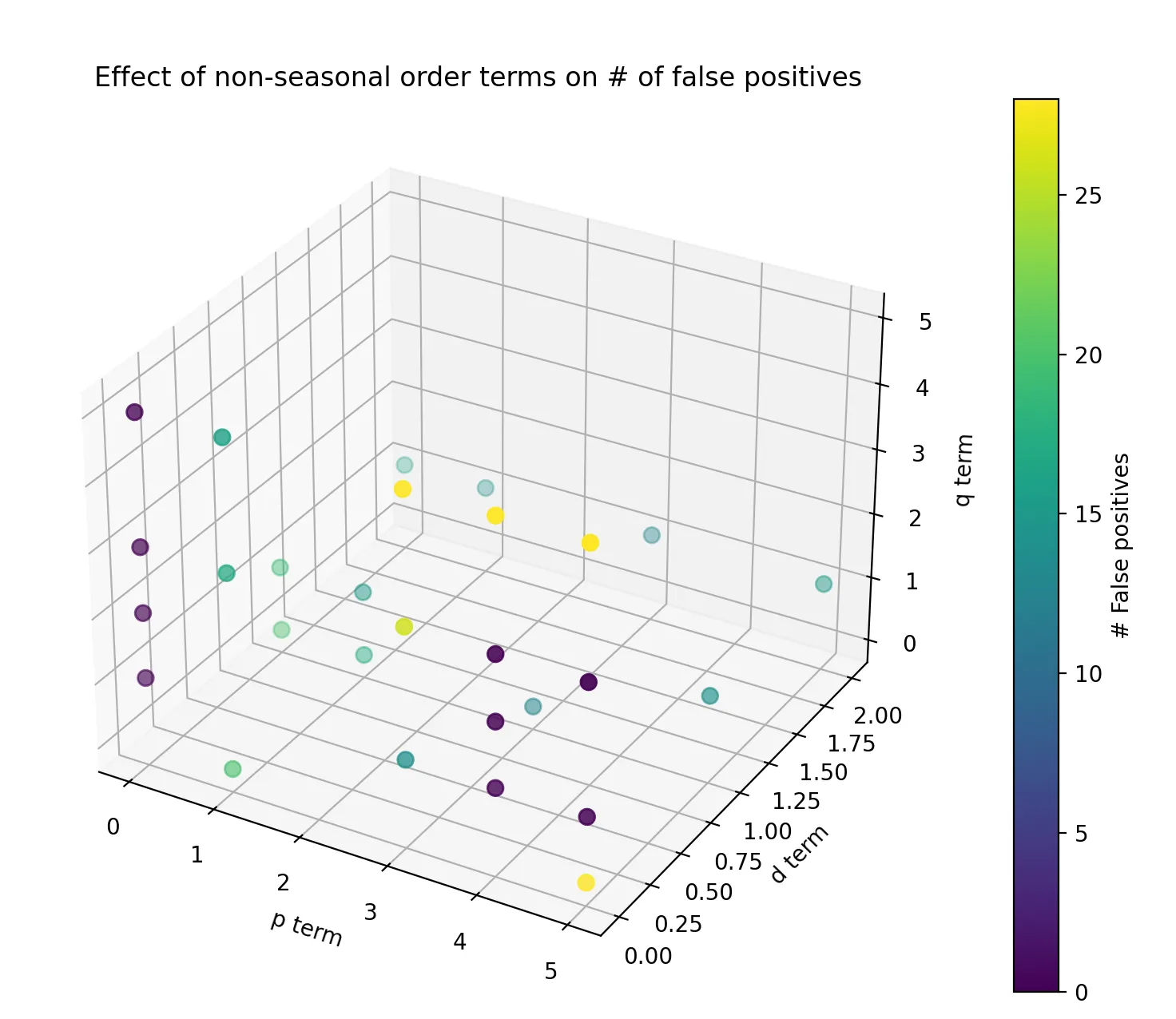
What we are most interested in is the combination which resulted in the lowest number of false positives. When bringing this back to our larger dataset, some of these combinations didn’t perform as well as the smaller experiment, but the best combination of values was p=0, d=0 and q=1 which corresponds to a moving average model. In our particular case, this provided the best results, but you should always fine-tune these values based on your application as this combination will not always be the best one!
Using this method, the number of false positives dropped to only 1 false positive (when using our optimisation from part 1 but not 2) and 9 false positives (when using both part 1 and 2).
Conclusion
Overall, when using BigQuery for numerical data, the algorithm is able to pick up on all intended anomalies with relative ease. The key concern is the number of false positives. In itself, it isn’t a terrible issue to have as you would rather over-estimate rather than under-estimate the number of anomalies when improving your data quality. However, it does makes things like automation more difficult, especially if you need to manually validate that a data point is not an anomaly.
By experimenting, we found that the best way to improve our utilisation of the BigQuery ML anomaly detector is by combining an increase in the threshold of what is considered an anomaly and fine-tuning the non-seasonal order terms. This resulted in a 95% decrease in the number of false positives.
If you liked this article, don’t hesitate to check out the first article in this anomaly detector series: Step-by-Step Guide to building an Anomaly Detector using a LLM and have a look at @ChloeCaronEng for more exploratory journeys!